Quicksort And Bubblesort Time Complexity

This week I was tasked to implement bubble sort and empirically calculate its time complexity. But first what even is time complexity?

Time complexity

In computer science, computational complexity indicates the amount of resources an algorithm needs to execute. The are two types of complexities:

• time complexity (computation time)
• space complexity (memory storage requirements)

In this post, I will only focus my attention on the former.

Time complexity provides an estimate of the amount of time an algorithm takes to run as a function of the size of its input. This estimate supposes that each elementary operation takes a fixed amount of time. Thus, the amount of time taken by the algorithm can be related by a constant factor.

Time complexity is often expressed using big O notation, which describes the upper bound on the growth rate of an algorithm’s running time as the size of the input increases.

Big O notation

Big O notation is a notation that describes the limiting behavior of an asymptotic growth rate of a function or an algorithm. It provides a way to classify the efficiency of algorithms in terms of their worst-case, best-case or average-case performance.

To put it formally:

$$ {\displaystyle f(x)=O{\bigl (}g(x){\bigr )}\quad {\text{ as }}x\to \infty } $$

• $f$ is the function we want to be estimated.
• $g$ is the comparison function.
• both functions are defined on some unbounded subset of real positive numbers $(+1,+2,+3,+4, …+\infty )$.
• $g(x)$ is stricly positive for all large numbers of $x$.

Now that we have a more formal explanation of Big O let’s look at this graph I found online:

![big_o_plane]We can see that as the number of elements increases, the growth rate stays constant but depending on our constant, the algorithm might scale linearly $O(n)$, others logarithmically $O(\log(n))$, and some even exponentially $O(n!)$.

Big O and algorithms

Now that we have a general idea of what Big O let’s see how we can apply it to algorithms so that we can quickly assess the time complexity of an algorithm.

Before going into bubble sort it’s better to cement the relationship between Big O and an algorithm.

So to do that let’s make a simple function that counts the even numbers inside an array.

def find_even_numbers(data: List[int]) -> int:
    counter = 0
    for i in data:
        if i % 2 == 0:
            counter += 1
    return counter

This function function iterates through the entirety of the list, if it finds an even number if i % 2 == 0: then it will increment our counter.

Because we are iterating over our entire array using our for loop, we can safely assume that our running time is $O(n)$. But let’s look at a graph.

To do that we first need an array of values and an array to store the times.

time_complexity = []
values = [1000, 5000, 10000, 50000, 100000, 500000, 1000000, 2000000,  3000000, 5000000]

for n in values:
    data = [random.randint(1, 1000) for i in range(n)]

    start_time = time()
    find_even_numbers(data)
    end_time = time()

    print("number finder time", end_time - start_time)
    time_complexity.append(end_time - start_time)

plt.plot(values, time_complexity, label="time complexity")
plt.grid(True)
plt.legend()
plt.show()

To empirically calculate the time complexity we create a list comprehension that iterates through the various values inside or array and creates an array of random integers of that specific size.

We then get the starting timestamp before and after executing the function and calculate the difference. To plot everything we use a library called matplotlib to create a plot and pass the array size as the X axis and the different timing as the Y axis.

This is the result:

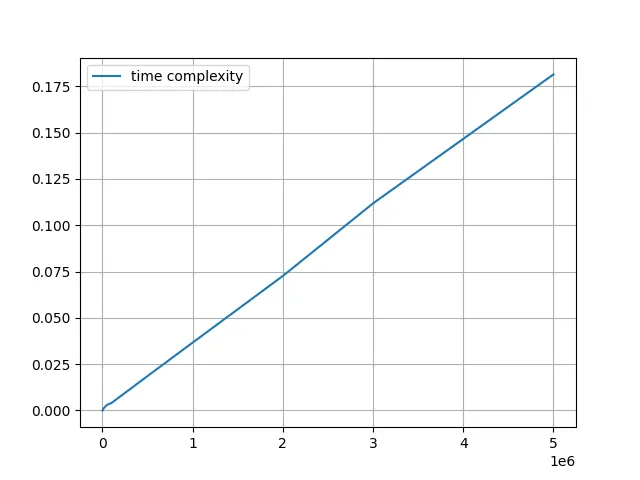
Yep, pretty linear. As the array size increases so does the time required to calculate the total amount of even numbers in that list.

Bubble Sort

Now that we have a basic understanding of time complexity and big O let’s look at bubble sort.

Bubble sort is a very simple sorting algorithm. It gets its name because out of every pass, the highest number in the list always reaches the top like a bubble reaching the surface of the water.

The algorithm is pretty simple.

• Iterate through the list
• if the first number is bigger than the one next to it, switch the place
• if the number is smaller, ignore them and go to the next pair of number
• rinse and repeat for the length of the array - 1 times.

Example

Let’s give an example:

If we have this list, [1, 5, 7, 3]

What bubble sort does is this:

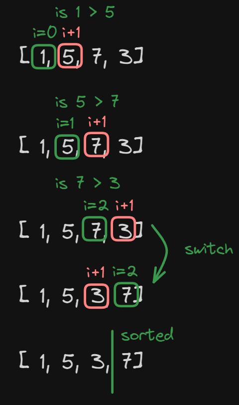
because the array is 4 units big, we are going to iterate over this array 4 - 1 = 3 times. The image shows what happens during the first pass.

• We start from the beginning of the array at position i = 0.
• We then get the element in the position i + 1.
• We compare if i > i + i.
• In this case, we see that at position i=0 we have the value 1 and at position i + 1 we have the value 5.

Now we check if 1 > 5, since it’s not we don’t do anything and move to the next pair.

In the case where i = 1 the same thing happens.

In the case of i = 2 we see that in position i = 2 we have the value 7 and in position i + 1 we have the value 5. So in this case the comparison is true and so we switch them place. At this point, we finished the first pass of the algorithm and now we have the value 7 at the very last place of our array.

Let’s look at the second pass:

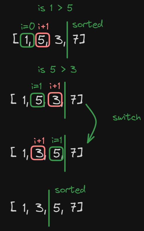
Because we already sorted the first biggest number there is no need to iterate over it, so we are going to have just two iterations.

Just like before we see that at position i=0 we have 1 and at position i + 1 we have the value 5. So again no switch.

At position i = 1 we have 5 and at position i + 1 we have the value 3. In this case, we switch. At this point, we have reached the end of the unsorted part of the array so we can move on to the last pass of the array. Remember 4 element array, 3 iterations.

Now the last pass of our algorithm.

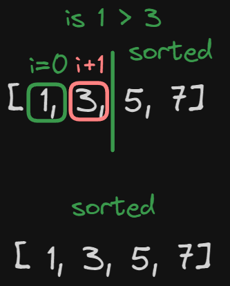
This last part is already sorted, so we check if 1 > 3, because it’s not, we don’t do anything and we reach the end of the unsorted part of the array, and now the whole array is sorted.

Code Implementation

Let’s implement this in the code now.

def bubble_sort(data):
    for i in range(len(data) - 1):
        for j in range(len(data) - 1 - i):
            if data[j] > data[j + 1]:
                data[j], data[j + 1] = data[j + 1], data[j]
                
    return data

That’s it!

What we are doing here is: in the first for loop for i in range(len(data) - 1): we want to iterate over the entire array size - 1. The reason why we doing it one less time than the array length is that when we do the n - 1 pass we have already sorted the array, so there is no need to do another pass.

The second nested loop for j in range(len(data) - 1 - i): Is the one that iterates over each element inside the array. To put it simply the images in the example represent an iteration of the first loop, while the actual comparison represents an iteration of the nested loop. (In retrospect I should have used j in the pictures to make it more clear, but oh well!).

Inside the for loop, we have this if statement, if data[j] > data[j + 1]: that checks if the value in potion j is bigger than the value in position j + 1. This last line data[j], data[j + 1] = data[j + 1], data[j]` simply swaps the two values.

The time complexity of bubble sort is $O(n^2)$ Let’s see why:

1. In the worst-case scenario, for each element in the list, bubble sort needs to compare it with every other element in the list. This results in $n$ comparison for the first item in the list, $n - 1$ for the second item, $n- 2$ for the third and so on until 1 comparison for the second-to-last element. $$ (n-1) + (n-2) + (n-3) + … + 2 + 1 $$ By using the sum of natural numbers formula we can rewrite the previous equation like this: $$ \sum_1^n{\frac{n(n+1)}{2}} $$

Due to the nature of Big O, we drop constants and remove the sum so the formula becomes this:

$$ n(n+1) $$

Let’s calculate this:

$$ n^2 + n $$

And now because in Big O, we can drop non-significant values we can do this: $$ (n^2 + n) \backsim n^2 $$

The reason why in Big O we can do that is because given a big enough value of $n$ the $ +n$ inside $n^2 +n $ doesn’t really matter.

Now let’s look at the time complexity on a graph.

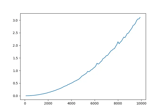
As you can see this graph clearly depicts a quadratic curve, more specifically this is a parabola $f(x) = ax^2 + bx + c $ with $x > 0$ because you can’t create an array with negative dimensions.

Quicksort

The quicksort is a divide-and-conquer algorithm. It works by selecting a ‘pivot’ element from the array and partitioning the other elements into two sub-arrays according to whether they are less than or greater than the pivot. The sub-arrays are then recursively sorted.

1. The first thing that needs to be done is choosing a pivot point.
   One can choose a pivot wherever their heart pleases but most commonly is the last element of the array.
2. The second thing that needs to be done is partitioning the array. This means re-arranging the array so that all the elements on the left side of the pivot are less than it and all the elements on the right side of the pivot are bigger than it. After partitioning, the pivot is in its final sorted position.
3. Now all we need to do is recursively apply steps 1 and 2 on the sub-arrays that have formed by partitioning.
4. Every recursive algorithm needs a base case and this algorithm is no exception. In this case the base case occurs when the sub-array size becomes 0 or 1, as a single-element array is already considered sorted.
5. Finally, the last step is to recombine the sub-arrays, which are sorted in place, but no explicit ‘combine’ step is needed. The entire array is sorted when the recursive calls finish.

Example

Let’s take the same array as before [1, 5, 7, 3] and sort it using quicksort:

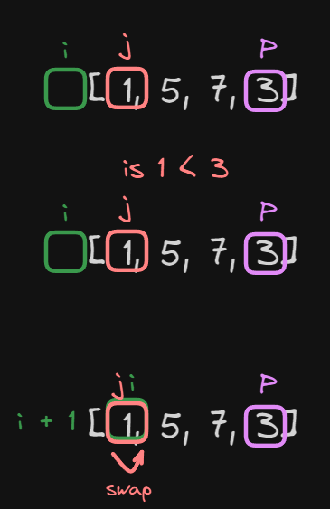
The first that is done here, is setting the pivot point highest element of the array. After that, we set the j element as the lowest element of the array and the i element as lo - 1, one less than the lowest element possible.

Now, we compare the element j with our pivot. In this case, we have the equation $1 < 3$, which is true. So what we do now is:

1. Increment i by 1
2. and swap the element j with the element j

In this case, both j and i point at the same value inside the array so even though we swapped values nothing changed.

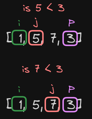
Now, we increment j by 1 and do the comparison again. Is $5 < 3$? This is false, so we don’t do anything and move on to the next iteration.

Let’s increment again j by 1 and do the comparison again.

Is $7 < 3$? This is again false, so we don’t do anything and move on to the next iteration.

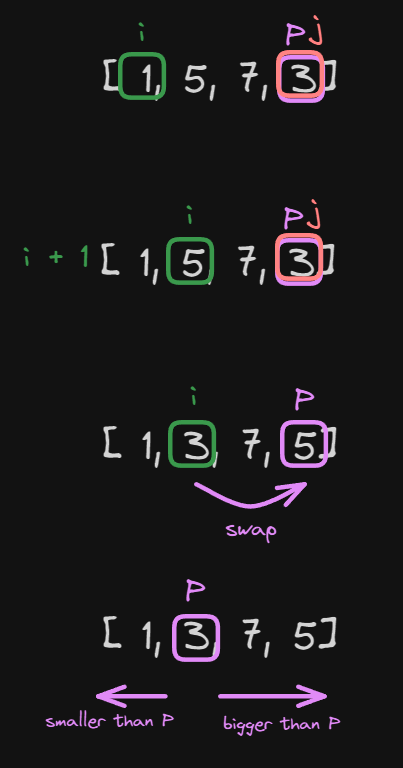
At this point, the value j is the same as our pivot. So to finish the first iteration of our quicksort algorithm we increment i by 1 and swap the place of the pivot with i. At this point, the first iteration is finished and we have successfully weakly sorted the array.

NOTE weakly sorted means that every value before the pivot is smaller and every value after the pivot is bigger, we don’t mind that for example 7 and 5 are not sorted yet, in the next iterations they will get sorted.

At this point, we reached the end of the quicksort algorithm. All we need to do now is break our arrays into sub-arrays and iterate our quicksort algorithm until we reach our base case.

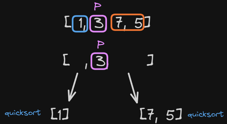
In this case, the first part of the sub-array is already sorted, because we only have one item (base case).

So let’s look at the other case:

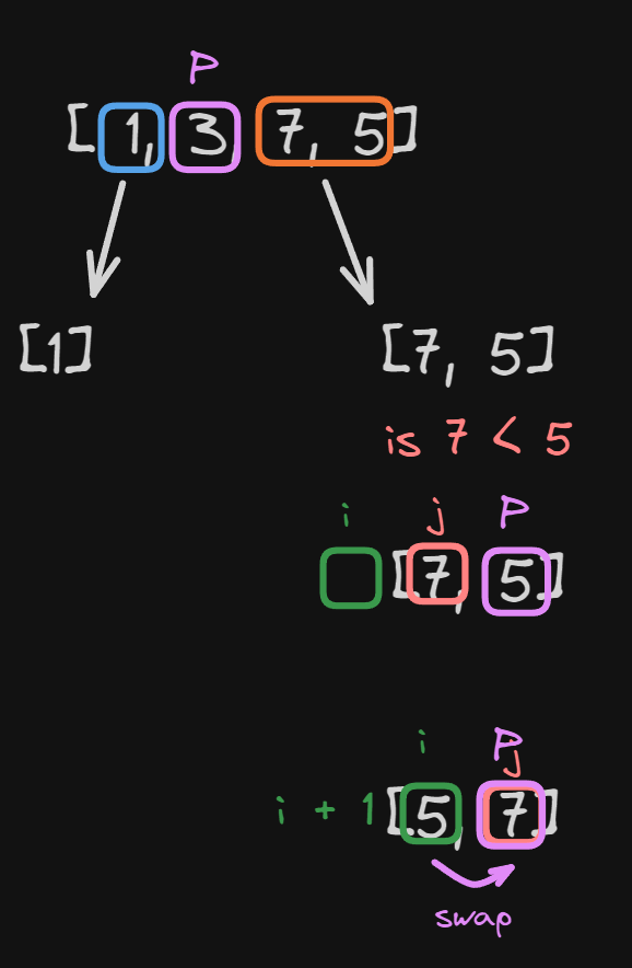
We have our array [7, 5]:

1. We chose the last element as our pivot.
2. We take the lowest point of the array as j.
3. i is 1 less than our lowest point.

Now we check if $7 < 5$, which is false, so we increment j

At this point, j and our pivot point are the same so we increment i by 1 and we swap i and our pivot

Now each sub-array is sorted so we just combine our sub-array into our original array.

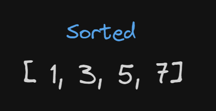
And ta-ah our array is sorted!

Implementation

To implement this algorithm we split it into two parts:

1. A partition method
2. A quick_sort method

Let’s first look at the partition method

Partition

def partition(data, lo, hi):
    pivot = data[hi]

    i = lo - 1
    for j in range(lo, hi):
        if data[j] < pivot:
            i  = i + 1
            data[i], data[j] = data[j], data[i]

    data[i + 1], data[hi] = data[hi], data[i + 1]
            
    return i + 1

To partition an array we need 3 variables:

1. The array itself (data).
2. the lowest point of the array (lo)
3. The highest point of the array (hi)

The first thing to do is to set our pivot to the last element of the array pivot = data[hi]. Then we instantiate i as the value of lo - 1.

Now we iterate using a for loop from the lowest value of the array to the highest for j in range(lo, hi): If the value inside j is less than the pivot we increase i by one and swap the data

        if data[j] < pivot:
            i  = i + 1
            data[i], data[j] = data[j], data[i]

After the for loop is finished we swap our pivot with i + 1.

data[i + 1], data[hi] = data[hi], data[i + 1]

Now let’s look at the quicksort method.

quicksort

def quick_sort(data, lo, hi):
    if lo <= hi:

        pivot = partition(data, lo, hi)

        quick_sort(data, lo, pivot - 1)
        quick_sort(data, pivot + 1, hi)

Just like the partition method we need 3 variables:

1. The array itself (data).
2. the lowest point of the array (lo)
3. The highest point of the array (hi)

if lo <= hi we start performing our algorithm. NOTE the equal is useless, I just like to include it lol.

Looking at our partition method we can see that at the end of the algorithm, it will return the new position of our pivot. So inside the quick_sort method, we will save that into a pivot variable.

Now just recursively call the quick_sort method for the sub-arrays before and after our pivot.

quick_sort(data, lo, pivot - 1)
quick_sort(data, pivot + 1, hi)

This code does what is described in the picture below:

And we are done with quicksort!

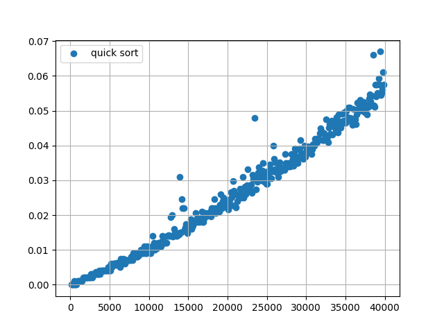
To finish this post let’s see its time complexity.

1. In the best-case scenario, Quicksort divides the array into approximately two equal parts at each step. This means that each partitioning step divides the array into two subarrays of roughly equal size. In this case, the algorithm achieves a time complexity of $O(n\log{n})$, where $n$ is the number of elements in the array. This occurs when the pivot element divides the array into two subarrays of roughly equal size at each step.

2. The average case of Quicksort also has a time complexity of $O(n\log{n})$. This assumes that the pivot selection process doesn’t consistently pick the worst possible pivot, leading to unbalanced partitions. In practice, Quicksort tends to perform well on average.

3. The worst-case scenario occurs when the pivot element is either the smallest or largest element in the array at each step, leading to highly unbalanced partitions. In this case, the algorithm behaves similarly to the insertion sort algorithm, resulting in a time complexity of $O(n^2)$. This worst-case scenario typically occurs when the array is already sorted or nearly sorted, and the pivot selection strategy isn’t optimized.

But why $O(n\log{n})$?

To calculate the time complexity we need to understand that the time complexity of quicksort we must have this formula in mind:

$$ T(N) = T(J) + T(N - J) + M(N) $$

• $T(N)$ is the complexity of quicksort for input size $N$
• $T(J)$ is the complexity of quicksort for input size $J$
• $T(N - J)$ is the complexity of quicksort for input size $N -J$
• $M(N)$ is the complexity of finding the pivot point for $N$ elements

In the best-case scenario we can say this: $T(N) = 2T(\frac{n}{2}) + const * n$ $2T(\frac{n}{2})$ is because the array is being divided into two arrays of equal size and $const * n$ is because each element of the array in each level of the tree is traversed.

Because the array will be divided into arrays of equal sides we will have this: $$ T(n) = 2(2T (\frac{n}{4} ) + const * (\frac{n}{2}) + const * n == 4*T(\frac{n}{4}) + 2 const * n $$

At this point we can say: $$ T(n) = 2^k * T(\frac{n}{2^k}) + k * const * n $$

Now we know that: $$ n = 2^k $$

So let’s find $k$: $$ k = \log_2{n} $$

Thenfore our final formula is: $$ T(n) = n * T(1) + n * \log{n} = O(n*\log_2{n}) $$

To finish with this post let’s see the time complexity graph: