12 minutes
Regression And Curve Fitting
In my last post, I explored two sorting algorithms and also discussed their time complexity, you can find it here. In this post, I want to piggyback off it and fit some curves on the empirical time complexity data that I collected.
Just like the last post, I will start with the function that scales linearly so that we can better grasp the concepts behind regression.
Linear Regression
Linear regression is a fundamental statistical method that is used to model a linear relationship between a dependent variable (usually Y) and one or more independent variables (usually X).
The general formula for linear regression is as follows:
$$ Y = \beta_0 + \beta_1 X + ε $$
Where:
- Y is the dependent variable (the variable we want to predict).
- X is the independent variable (the variable used to make predictions).
- $\beta_0$is the intercept (the value of $Y$ when $X=0$).
- $\beta_1$ is the slope (the change in $Y$ for a one-unit change in $X$).
- $ε$ is the error term, representing the difference between the observed $Y$ and the predicted $Y$.
The goal of linear regression is to estimate the coefficients $\beta_0$ and $\beta_1$ that best fit the observed data. This is typically done by minimizing the sum of squared differences between the observed and predicted values of $Y$, a method known as the least squares approach.
Personally I don’t love using $\beta_0$ and $\beta_1$ and I prefer the nomenclature that I am most familiar with, which is:
$$ y = m x + b $$
- $m$ is the slope of the function.
- $b$ is the $y$ intersect.
When removing ε from the first equation, we can see that the two equations both represent a straight line in a planar space.
Calculating the error
To calculate the error we will use a method known as the least squares approach.
Let’s look at an example before we see the formula:
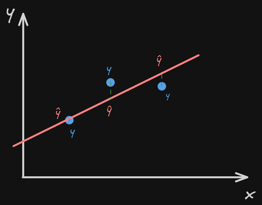 In this image, we are trying to fit a line so that the sum of all the distances of the 3 points is as small as possible.
We can see that the distance is showing as a green dotted line that goes from $y$ which is the real $y$ and $\hat{y}$ which is the estimated value of $y$.
At this point, in order to avoid negative values that would ruin the result of our sum (this happens when $\hat{y}$ is sitting above $y$), we square the error.
In this image, we are trying to fit a line so that the sum of all the distances of the 3 points is as small as possible.
We can see that the distance is showing as a green dotted line that goes from $y$ which is the real $y$ and $\hat{y}$ which is the estimated value of $y$.
At this point, in order to avoid negative values that would ruin the result of our sum (this happens when $\hat{y}$ is sitting above $y$), we square the error.
If we were to visualize it, it would look like this:
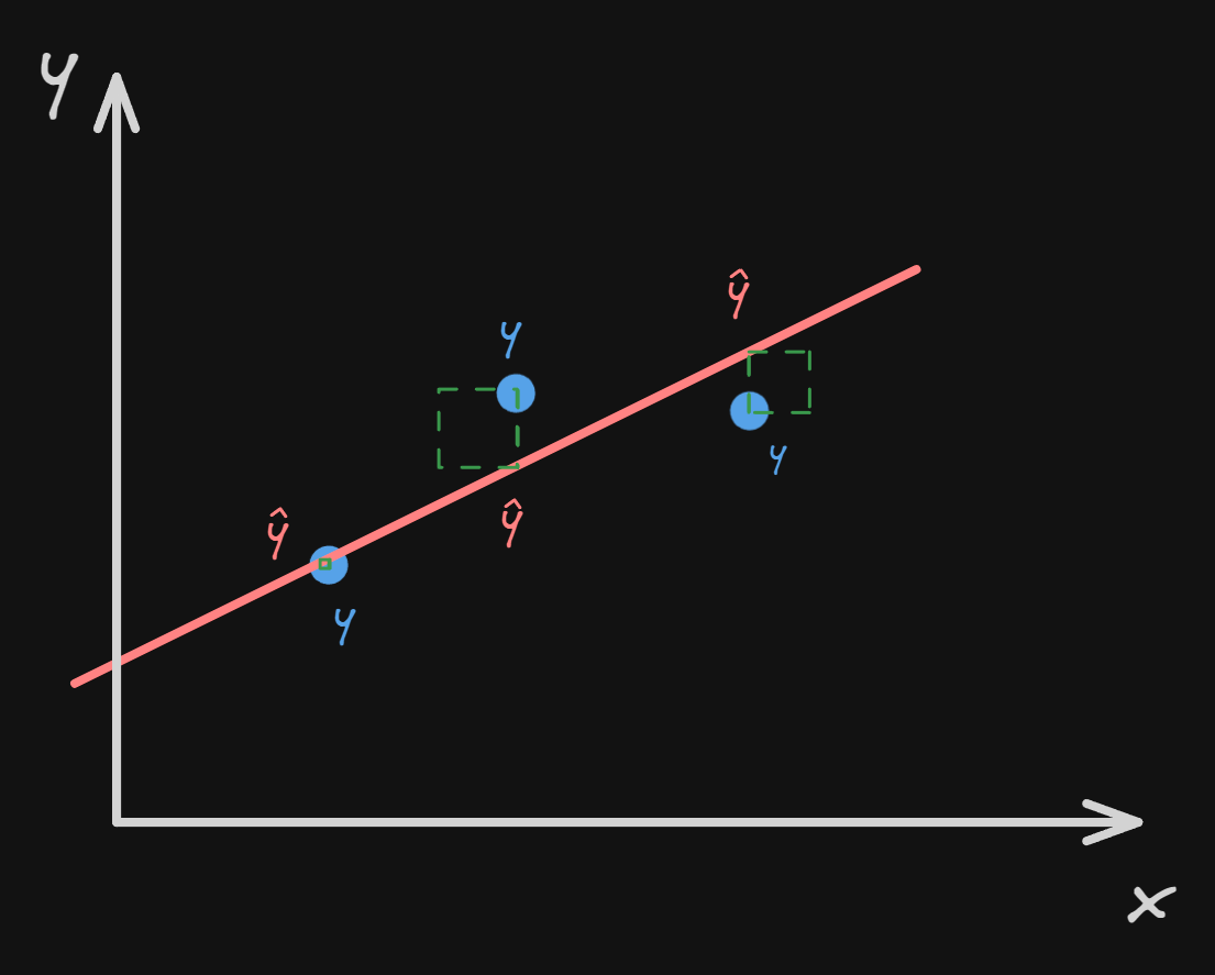
The formula for finding the square error for one point is:
$$ E = (y - \hat{y})^2 $$
Because we are dealing with many points we should turn this into a sum:
$$ E = \frac{1}{n} \sum_{i=0}^{n}(y_i - \hat{y}_i)^2 $$
NOTE: If you are wondering why I also added $\frac{1}{n}$ it’s because we need to normalize the sum of the squared errors to the numbers of observations. Without it, the mean square error would increase as the numbers of datapoints increases, making it difficult to compare models.
This $\hat{y}$ may seem complicated to understand but its basically a specific point inside our linear equation. This means we can re-write the mean square equation as such:
$$ E = \frac{1}{n} \sum_{i=0}^{n}(y_i - (mx_i + b))^2 $$
Minimizing the error
Now that we can calculate the error of our line using the mean square error, how do we go about minimizing it.
$$ y = m x + b $$
By looking at our linear equation we can see that we can modify two parameters
- $m$
- $b$
If you are familiar with calculus this is quite obvious, all we need to do is to find the derivative of the function and set it to zero. Because we have two variables, we need to use multivariable calculus, that means partial derivatives.
In the case of linear regression this approach does make sense, but when you are dealing with high-dimensional feature spaces calculating the normal equation involves computing the inverse of a matrix, which can be computationally expensive. So, for this example, we will use a technique called gradient descent, which is more efficient, especially in big datasets and doesn’t involve matrix inversion.
Gradient descent
The general idea of gradient descent is to tweak parameters iteratively in order to minimize a cost function.
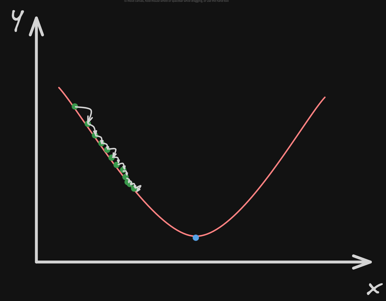
To better understand how gradient descent works, we can imagine that we are lost in the mountains and it’s pitch black, we can’t see anything! We want to go home, this means going back to the bottom of the mountain. A good strategy is to make tiny steps and feel with our feet and follow the steepest slope of the mountain. This is gradient descent! It measures the local gradient of the error function about the parameter vector θ(The parameters of the linear regression model (θ) are typically represented as a vector), and it goes in the direction of a descending gradient. Once the gradient reaches zero, we have reached a minimum.
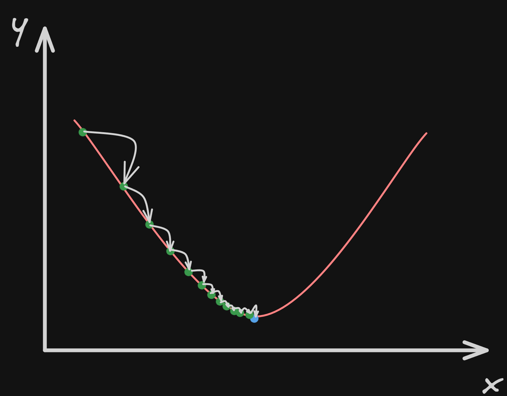 In this graph, we can imagine the the axis $y$ is the altitude of the mountain, and the axis $x$ is us moving in one direction.
At this point let’s look at our error function and find the gradient:
$$ E = \frac{1}{n} \sum_{i=0}^{n}(y_i - (mx_i + b))^2 $$
So to solve this we need to take the partial derivate with respect to $m$ and $b$.
$$ \frac{\partial E}{\partial m} = - \frac{2}{n} \sum_{i=0}^{n} x_i (y_i -(m x_i +b)) $$
$$ \frac{\partial E}{\partial b} = - \frac{2}{n} \sum_{i=0}^{n} (y_i -(m x_i +b)) $$ At this point, we can calculate the direction of the steepest ascent.
To calculate what we actually want, we simply put a minus in front of it.
To improve $m$ in this case all we need to do is to:
$$ m = m - L * \frac{\partial E}{\partial m} $$ We are taking $m$ and assigning it $m$ minus $L$ which is the learning rate, multiplied by the direction of the steepest ascent $\frac{\partial E}{\partial m}$.
The same is done for the parameter $b$:
$$ b = b - L * \frac{\partial E}{\partial b} $$
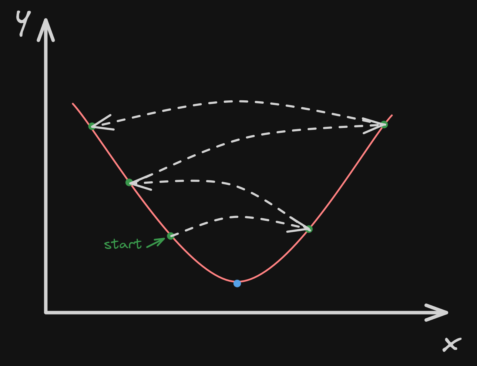
The learning rate $L$ is a hyperparameter used in gradient descent. If the learning rate is too small, then the algorithm will have to go through many iterations to converge, which will take a long time.
On the other hand, if the learning rate is too high, we might jump across the valley and end up on the other side, possibly even higher up than we were before. This might make the algorithm diverge.
Implementing Linear Regression
Now that we understand how linear regression and gradient descent work let’s implement them in Python so that we can find
the best curve to represent our method find_even_numbers that I showed in the previous blog post.
In the previous example, we created a piece of code that counted the amount of even numbers in an array and we plotted the time needed to execute based on different array sizes. The resulting graph is like this:
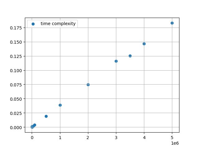
Now let’s implement linear regression to find the best fitting line:
def loss_function(m, b, x_data, y_data):
    total_error = 0
    for i in range(x_data):
        x = x_data[i]
        y = y_data[i]
        total_error += (y - (m * x + b)) ** 2
    total_error / float(len(x_data))
This is the loss function, we initialize the variable total_error to zero and then we iterate through
two arrays, x_data and y_data that represent the two axes.
to get the sum of the errors we have written the previously shown formula in a Pythonic way.
In the end, to get the mean squared error, we divide by the length of the data.
This method that I included is only for educational purposes only because the gradient descent method already includes the partial derivatives for the mean square function.
def gradient_descent(m_now, b_now, x_data, y_data, L):
    m_gradient = 0
    b_gradient = 0

    n = len(x_data)

    for i in range(n):
        x = x_data[i]
        y = y_data[i]

        m_gradient += -(2/n) * x * (y - (m_now * x + b_now))
        b_gradient += -(2/n) * (y - (m_now * x + b_now))

    m = m_now - m_gradient * L
    b = b_now - b_gradient * L

    print("inside the gradient", m, b)
    return m, b
This function iterates over the entire array and calculates the gradient for $m$ $b$ and at the end of the loop it sets the values of $m$ and $b$ to be $m$ minus the gradient multiplied by the leaning factor.
m = 0
b = 0
L = 0.0000000000001

epoch = 10000

for i in range(epoch):
     m, b = gradient_descent(m, b, values, time_complexity, L)

print(m, b)

plt.scatter(values, time_complexity, label="time complexity")
plt.plot(values, [m * x + b for x in values], color='red')

plt.grid(True)
plt.legend()
plt.show()
To call the gradient_descent method we must first set the variables.
$m = 0$, $b = 0 $ $L = 0.0000000000001$, and the epoch = 10000 (epoch is a fancy word for several iterations).
By setting $m$ and $b$ to zero we essentially created a straight line, parallel to x with intersect at $y = 0$ we created a line on top of the x-axis.
The reason why the learning rate is so small is that even for relatively a 5000000-size array it takes less than a second to compute.
NOTE: I’ve tried to make the learning rate bigger but it diverges after some hundreds of iterations.
After running the code this is the final curve:
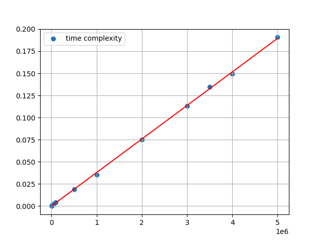
We successfully managed to fit our curve and now we can see that in our linear equation has a slope of $m =3.79133470400 * 10^{-8}$ and y intersect of $b = -2.197994308940 * 10^{-13}$.
Polinomial Regression
Now that we can manage to fit linear curves to points let’s step it out a notch by fitting polynomials in our data points!
Let’s look at our first polynomial regression:
$$ Y = \beta_0 + \beta_1 X + ε $$
Looks familiar? That is because technically speaking the vanilla linear regression is also a polynomial regression. More specifically linear regression is a first-order polynomial regression.
Now let’s look at a second-order polynomial regression:
$$ Y = \beta_0 + \beta_1 X + \beta_2 X^2+ ε $$ Basically, for every order of our regression we add a $b_k$ value and an $x^k$ variable. To generalize:
$$ Y = \beta_0 + \beta_1 X + \beta_2 X^2+ … + \beta_k X^k + ε $$
Now you might be wondering how can we fit this linear model with all these non-linear terms. Well, the important thing to remember is that we just care about the coefficients, not the variables. If we take a look at our formula all the coefficients are linear, this means this is s standard linear model!
One thing to note that I won’t be discussing in this blog post is how can we know which order should we stop when we have no idea what the order might be. To pick the optimal model we use the Bayesian Information Criterion (BIC).
Calculating the error
To minimize the error in our curve we take the same mean square error formula as before
$$ E = \frac{1}{n} \sum_{i=0}^{n}(y_i - \hat{y}_i)^2 $$
but now in $\hat{y}$ we substite the quadratic formula $ax^2 + bx + c$.
$$ E = \frac{1}{n} \sum_{i=0}^{n}(y_i - (ax^2 + bx +c))^2 $$
Minimizing the error
To minimize it now, we simply perform the gradient descent method again and derive this equation with respect to $a$, $b$, $c$:
$$ \frac{\partial E}{\partial a} = - \frac{2}{n} \sum_{i=0}^{n} x_i^2 (y_i -(a x_i^2 +bx +c)) $$
$$ \frac{\partial E}{\partial b} = - \frac{2}{n} \sum_{i=0}^{n} x_i (y_i -(a x_i^2 +bx +c)) $$
$$ \frac{\partial E}{\partial c} = - \frac{2}{n} \sum_{i=0}^{n} (y_i -(a x_i^2 +bx +c)) $$
To minimize the error we now have to improve these 3 values $a$, $b$, $c$:
$$ a = a - L * \frac{\partial E}{\partial a} $$ $$ a = b - L * \frac{\partial E}{\partial b} $$ $$ c = c - L * \frac{\partial E}{\partial c} $$
Implementing Linear Regression
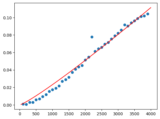
We will now implement the bubble_sort algorithm that I showed in the previous post.
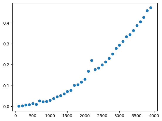
From this picture, it’s pretty clear that we are dealing with a quadratic equation. So let’s create a gradient descent function for quadratic equations:
def quad_gradient_descent(a_now, b_now, c_now, x_data, y_data, L):
    a_gradient = 0
    b_gradient = 0
    c_gradient = 0

    n = len(x_data)

    for i in range(n):
        x = x_data[i]
        y = y_data[i]

        a_gradient += -(2/n) * x ** 2 * (y - (a_now * x**2 + b_now * x + c_now))
        b_gradient += -(2/n) * x * (y - (a_now * x**2 + b_now * x + c_now))
        c_gradient += -(2/n) * (y - (a_now * x**2 + b_now * x + c_now))

    a = a_now - a_gradient * L
    b = b_now - b_gradient * L
    c = c_now - c_gradient * L

    return a, b, c
This function returns our three optimized parameters in a tuple $a$, $b$, $c$.
Now let’s initialize our values, set the learning rate and show our plot:
a = 0
b = 0
c = 0
L = 0.00000000000001

epochs = 10000

for i in range(epochs):
    a, b, c = quad_gradient_descent(a, b, c, values, bubble_time_complexity, L)

print(a, b, c)

plt.scatter(values, bubble_time_complexity)
x_range = np.linspace(0, 4000, 100)
quadratic_curve = a * x_range**2 + b * x_range + c
plt.plot(x_range, quadratic_curve, color="red")
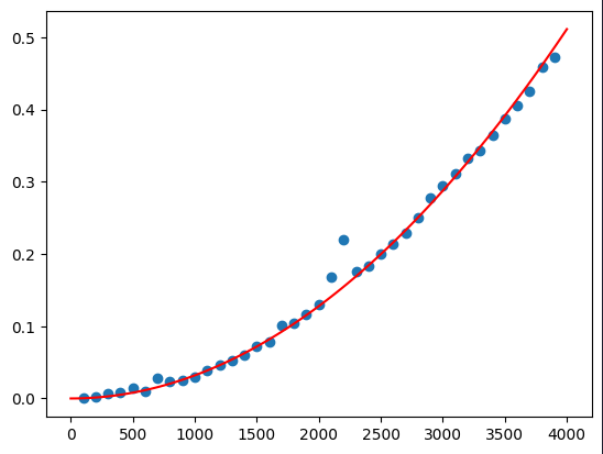
We successfully managed to fit our curve and now we can see that our parabola has $a =3.19418* 10^{-8}$, $b = 5.79448 * 10^{-10}$ and $c = 5.01148 * 10^{-13}$.
Fitting a logarithm
Fitting a logarithm is no different from fitting any type of polynomial because, again, all the coefficients are still linear!
To fit the time complexity of the last algorithm quick_sort we need an equation of type:
$$ Y = \beta_0 X * \log(X) + \beta_1 $$
Let’s implement our gradient descent again:
def x_log_gradient_descent(a_now, b_now, x_data, y_data, L):
    a_gradient = 0
    b_gradient = 0

    n = len(x_data)

    for i in range(n):
        x = x_data[i]
        y = y_data[i]

        # Compute gradients
        a_gradient += -(2/n) * x * np.log(x) * (y - (a_now * x * np.log(x) + b_now))
        b_gradient += -(2/n) * x * (y - (a_now * x * np.log(x) + b_now))

    # Update parameters using gradients and learning rate
    a = a_now - a_gradient * L
    b = b_now - b_gradient * L

    return a, b
Now, initialize the learning rate and our parameters:
a = 0
b = 0
L = 0.000000001

epochs = 100000

for i in range(epochs):
    a, b = x_log_gradient_descent(a, b, values, quick_time_complexity, L)

print(a, b)
We get our resulting parameters to be $3.3565* 10^{-6}$ and $3.5767 * 10^{-5}$.
Now by plotting it:
plt.scatter(values, quick_time_complexity)
a_range = np.linspace(100, 4000, 100)
log_curve = a * x_range * np.log(x_range) + b
plt.plot(x_range, log_curve, color="red")
We get our curve that best first our data, given the learning rate and epoch.